Warning

You're reading an old version (v5.2) of this documentation. If you want up-to-date information, please have a look at master.

Data Uncertainties

The data uncertainties, often referred to as the error bars, are critical in EM inversion since the data misfit and inversion search directions are both scaled by the data uncertainties. The error bars are just as important as the data! While most EM data and uncertainties are estimated as complex numbers in data processing codes, the complex values are often transformed into other forms for inversion (e.g., real, imaginary, amplitude, phase, log10 amplitude, apparent resistivity etc). Here we provide a table showing how to correctly scale the data uncertainties for each data type supported by MARE2DEM. For the interested reader, we also provide a brief review of the uncertainty propagations for the various transforms. For more details and discussion of some of the advantages and disadvantages of the various data scalings, see [WCK15].

Data Type

Data

Standard Error

complex

\(z=x+iy=ae^{i\phi}\)

\(\delta z = \sqrt{2} \sigma\)

real or imaginary

\(x,y\)

\(\delta x = \delta y = \sigma\)

amplitude

\(a = |z|\)

\(\delta a = \sigma\)

log10(amplitude)

\(l = \log_{10}|z|\)

\(\delta l=\frac{1}{\ln(10)}\frac{\sigma}{a}\)

apparent resistivity

\(\rho_a =\frac{1}{\omega\mu}|z|^2\)

\(\delta \rho_a = \frac{2 \rho_a}{|z|} \sigma\)

log10(app.resist.)

\(\log_{10}\rho_a\)

\(\delta \log_{10}\rho_a=\frac{1}{\ln(10)}\frac{\delta \rho_a}{\rho_a}\)

phase

\(\phi= \arctan(y/x)\)

\(\delta \phi=\frac{\sigma}{a}=\frac{1}{2}\frac{\delta\rho_a}{\rho_a}\)

Note that MARE2DEM inverts phase with units degrees, so multiply the phase and its uncertainty defined above by \(180/\pi\).

Complex Data

The complex data \(z = x + i y\) can be related to amplitude a and phase \(\phi\) (in radians) using Euler’s formula:

\[\begin{eqnarray} z = x + i y = a e^{i\phi} = a (\cos \phi + i \sin \phi), \end{eqnarray}\]

where

\[\begin{split}\begin{eqnarray} x &=& a \cos \phi, \\ y &=& a \sin \phi. \end{eqnarray}\end{split}\]

Likewise, the amplitude and phase can be found from the complex components using

\[\begin{split}\begin{eqnarray} a &=& \sqrt{x^2+y^2}, \\ \tan \phi &=& \frac{y}{x}, \\ \phi &=& \arctan \frac{y}{x}. \end{eqnarray}\end{split}\]

When computing \(\phi\), you should use the \(\it atan2(y,x)\) function since it returns the four-quadrant phase whereas the \(\it atan(y/x)\) function is restricted to \(-\pi \le \phi \le \pi\).

Also, when dealing with real data, we generally convert phase into degrees:

\[\begin{eqnarray} \phi (degrees)= \frac{180}{\pi} \phi (radians) \end{eqnarray}\]

Real and Imaginary

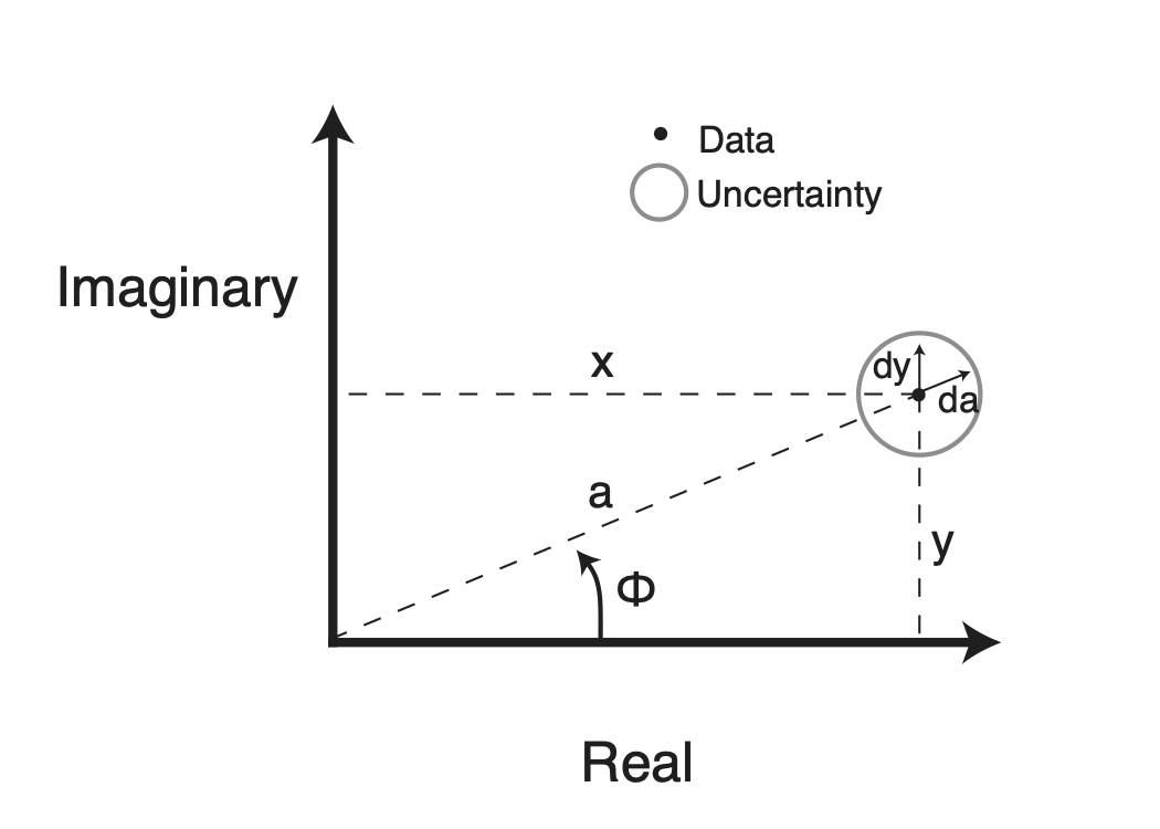
For complex data \(z = x + i y\) where x is the real component and y is the imaginary component, the standard error \(\sigma\) is generally assumed to be isotropic so that \(\sigma = \delta x = \delta y\). Isotropic error means that z has a circle of uncertainty around it in the complex plane as shown in Fig. 43.

_images/complex_errors.png

Fig. 43 Isotropic uncertainty in the complex plane

For CSEM data, z is the complex electric or magnetic field at a given frequency. For MT data, z is a component of the MT impedance tensor (or a component of the tipper vector) at a given frequency. In both cases, complex data z is what is output from the EM response estimation code that process the time series data.

MARE2DEM allows us to invert the data as a complex quantity, but often we find it more intuitive to look at the data in amplitude and phase form, or log(amplitude) and phase. In the case of MT, the apparent resistivity form is much easier to comprehend visually than the complex data z. When inverting CSEM and MT responses with a large dynamic range (i.e. spanning multiple orders of magnitude), there are some stability advantages to treating the data as log10(amplitude); see [WCK15].

Given a data scaling transform, we have to know the associated data uncertainty transforms. Suppose q is the transformed version of the original complex data z. Thus \(q \equiv q(x,y)\). For example, q could be the amplitude, phase, log(amplitude), apparent resistivity, a polarization ellipses parameter, etc. For computing misfits during modeling and inversion, we need to know the uncertainty \(\delta q\). This can be found using the standard method for linear propagation of errors, which uses a first-order Taylor’s series expansion. Assuming the variables x and y are independent with standard error \(\sigma\), the first-order variance propagation formula is

(4)\[\begin{eqnarray} \delta q^2 = \left ( \frac{\partial q}{\partial x} \right) ^2 \sigma^2 + \left ( \frac{\partial q}{\partial y} \right) ^2 \sigma^2. \end{eqnarray}\]

The sections below show how to apply this for the various data types supported in MARE2DEM.

Amplitude

The amplitude a of complex variable z is:

\[\begin{eqnarray} a = |z| = \sqrt{x^2+y^2}, \end{eqnarray}\]

Thus we have

\[\begin{eqnarray} \frac{\partial a}{\partial x} = \frac{x}{a}, \;\;\;\;\;\;\; \frac{\partial a}{\partial y} = \frac{y}{a}, \end{eqnarray}\]

Using eq. (4), we find

\[\begin{split}\begin{eqnarray} \delta a^2 &=& \left ( \frac{x}{a}\right )^2 \sigma^2 + \left ( \frac{y}{a}\right )^2 \sigma^2 ,\\ &= &\sigma^2. \end{eqnarray}\end{split}\]

The standard error is therefore

\[\begin{eqnarray} \delta a &=& \sigma . \end{eqnarray}\]

In Fig. 43 you can see that this result makes sense since \(\delta a = \sigma = \delta x = \delta y\).

log10 Amplitude

Warning

The standard error of log scaled data is not the log of the linear standard error!

Denote the log of the amplitude as variable l:

\[\begin{eqnarray} l= \log_{10}|z| = \log_{10}(a) = \log_{10}\left ( \sqrt{x^2+y^2} \right ). \end{eqnarray}\]

Using the chain rule we have

\[\begin{eqnarray} \frac{\partial l}{\partial x} = \frac{ \partial l}{ \partial a} \frac{\partial a}{\partial x} = \frac{1}{\ln(10) a} \frac{x}{a} = \frac{ x }{\ln(10) a^2}, \end{eqnarray}\]

with a similar expression for the y derivative.

Using eq. (4), the variance of l is then:

\[\begin{split}\begin{eqnarray} \delta l^2 &=& \left ( \frac{ x }{\ln(10) \, a^2} \right )^2 \sigma^2 + \left ( \frac{ y }{\ln(10)\, a^2} \right )^2 \sigma^2, \\ &= & \frac{\sigma^2}{\ln(10)^2\, a^2}. \end{eqnarray}\end{split}\]

The standard error of l is then:

\[\begin{eqnarray} \delta l &=& \frac{1}{\ln(10)} \frac{\sigma }{a} = 0.4343 \frac{\delta a }{a} . \end{eqnarray}\]

This shows that the standard error for the log10 scaled amplitude is just a scaled version of the relative amplitude error \(\frac{\delta a }{a}\). So if we say the data has 1% error in amplitude, the standard error of the log10 amplitude is then 0.004343.

It can also be helpful to think of visualizing the error bars on a log10 scaled plot of the amplitudes. The formula above shows that if the data have a fixed relative error, the error bars on the plot will all have the same vertical length, regardless of the data values.

Apparent Resistivity

The MT apparent resistivity \(\rho_a\) is found from the impedance \(Z = x + i y\) as

\[\rho_a = \frac{1}{\omega \mu} |z|^2 = \frac{1}{\omega \mu} (x^2+y^2)\]

Using the chain rule we have

\[\begin{eqnarray} \frac{\partial \rho_a}{\partial x} = \frac{2 x}{\omega \mu} \end{eqnarray}\]

and similarly for the y derivative. The standard error of \(\rho_a\) is then:

\[\delta \rho_a = 2 \frac {\sigma }{|Z|} \rho_a\]

and the relative error in apparent resistivity is

\[\frac{\delta \rho_a}{\rho_a} = 2 \frac{\sigma }{|Z|}\]

which is twice the relative error in the impedance, where the factor of two is due to the apparent resistivity being proportional to the square of the impedance magnitude.

Phase

The phase \(\phi\) of z in degrees is:

\[\begin{eqnarray} \phi = \frac{180}{\pi} \arctan(z) = \frac{180}{\pi} \arctan\left (\frac{y}{x} \right ), \end{eqnarray}\]

with partial derivatives

\[\begin{split}\begin{eqnarray} \frac{\partial \phi}{\partial x} &=& -\frac{180}{\pi} \frac{1}{1 + \left (\frac{y}{x}\right)^2} \frac{y}{x^2} ,\\ &=& -\frac{180}{\pi} \frac{y}{x^2 + y^2} . \end{eqnarray}\end{split}\]

and

\[\begin{eqnarray} \frac{\partial \phi}{\partial y} &=& \frac{180}{\pi} \frac{x}{x^2 + y^2} . \end{eqnarray}\]

Using eq. (4), we find

\[\begin{split}\begin{eqnarray} \delta \phi ^2 &=& \left (-\frac{180}{\pi} \frac{y}{x^2 + y^2} \right )^2 \sigma^2 + \left (\frac{180}{\pi} \frac{x}{x^2 + y^2} \right )^2 \sigma^2, \\ &=& \left ( \frac{180}{\pi} \right ) ^2 \frac{\sigma^2}{a^2} \end{eqnarray}\end{split}\]

The standard error of \(\phi\) is then:

\[\begin{eqnarray} \delta \phi &=& \frac{180}{\pi} \frac{\sigma }{a} =\frac{180}{\pi} \frac{\delta a }{a} = \frac{180}{\pi} \frac{1}{2}\frac{\delta \rho_a}{\rho_a} \end{eqnarray}\]

So for 1% relative error in amplitude (\(\frac{\delta a }{a}\)), the corresponding phase error \(\delta \phi\) is then 0.573º. Note also that the last term on the right shows the phase error for MT data will be half the relative error in apparent resistivity.

In Fig. 43 you can see that this result makes sense, since small changes in \(\phi\) will scale with \(\frac{\delta a }{a}\).

A word of warning

The uncertainty propagation analyses above relied on a first-order Taylor’s series expansion that implicitly assumes \(\sigma << |z|\), in other words it assumes that the uncertainty is much smaller than the data amplitude. The formulas for transformed uncertainties break down when the uncertainty grows too large. See [WCK15] for an in-depth analysis of the break-down. Hence, data with large errors (say greater than 50% or so) should generally be omitted from the inverted data set given issues with propagating the error; furthermore very noisy data probably doesn’t help the inversion resolve conductivity so it can have little useful value, that is unless the noisy data are all you have to work with.