Warning You're reading an old version (v5.0) of this documentation.
If you want up-to-date information, please have a look at master.
Bounding Inversion Parameters with Non-linear Transforms
Note
Global bounds on all model parameters can be set in the Mamba2D.m user interface that makes the Resistivity File (.resistivity), or you can hand adjust them in the file by modifying the line:
Global Bounds: 1.0000E-01, 1.0000E+05
where the values given are the lower and upper bounds (given in linear ohm-m). You can also specify which transform method to use in the Resistivity File (.resistivity) by including the line:
Bounds Transform: bandpass options: exponential or bandpass
Each individual free parameter given in the regions list section at the bottom of the .resistivity file can have its own specific lower and upper bounds specified (and this will override the global bounds set above). See Resistivity File (.resistivity).
The text below gives background theory on how the bounds are implemented in MARE2DEM. The model update equation (3) does not place any constraints on the range of values that a parameter can take, yet often there are geological reasons or ancillary data sets that suggest the conductivity will be within a certain range of values. When such inequality constraints are desired, they can be implemented simply by recasting the inverse problem using a non-linear transformation of the model parameters so that the objective function and optimization algorithm remain essentially the same as the unconstrained problem . The model parameter \(\mathbf{m}\) is bounded as
where l is the lower bound and u is the upper bound. The transformed parameter \(\mathbf{x}\) is unbounded:
With the transformed model vector \(\mathbf{x}\), the model update is accomplished with a modified version of (3):
where
(here the model prejudice term has been omitted for brevity). Thus the inversion solves for the unbounded parameter \(\mathbf{x}\) which can have values anywhere from negative to positive infinity. However the forward operations are carried out on the bounded parameter via \({F}(\mathbf{m(x)})\).
MARE2DEM (like most other EM inversions) already uses such a transform approach, in this case a one-sided bound by inverting for \(\log_{10} \rho\) to avoid physically meaningless negative resistivity (and conductivity). MARE2DEM also offers two additional types of bounding transforms that can be used constrain the range of resistivity for any given free parameter: the exponential and bandpass transforms. These are shown in the figure below and the text that follows explains the math behind these transforms.
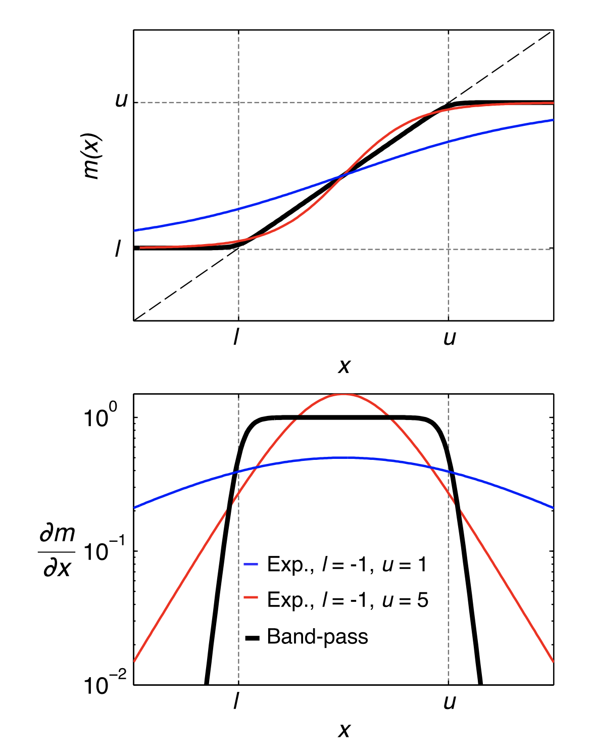
Fig. 44 Non-linear transforms used to bound model parameters during inversion. The bound model parameter function \(m(x)\) (top) and the sensitivity \(\frac{\partial m} {\partial x}\) scaling (bottom) are shown for the exponential transform (red and blue) and the bandpass transform (black). The bandpass transform was designed so that within the bounds, the transformed parameter (and its sensitivity) is nearly identical to the unbound parameter.
Both the exponential and band-pass transforms have been implemented in MARE2DEM so that each model parameter can have its own unique bounds specified. For some data sets the user will have a priori knowledge that can guide the use of a narrow range of parameter bounds in certain localized regions, for example where nearby well logs provided independent constraints on conductivity. Narrow bounds could also be prescribed to test hypotheses about the range of permissible resistivity values that fit a given data set. Yet in most cases the inversion will be run without any bounds. However, experience has shown there to be a benefit from applying global bounds on all model parameters so that extreme values are excluded from the inversion. In particular, if the line search jumps to very low \(\mu\) values, the Occam model update can produce rough models that have unrealistically high and low resistivity that usually produce poor misfit. Bounding all parameters to a plausible range (such as 0.1 to 100,000 ohm-m for marine models) alleviates this situation. Another consequence is that unrealistically conductive regions can cause the adaptive mesh refinement scheme in the forward code to spend excessive effort refining the mesh to produce accurate responses in these regions; bounding all the model parameters to a plausible range avoids this computational time-wasting situation.
Exponential Transform
The exponential transform is
For large positive \(x, m(x)\) asymptotes to \(u\), while for large negative \(x, m(x)\) asymptotes to \(l\). The sensitivity transform is found by taking the derivative of this expression, yielding:
The transformed variable \(x(m)\) can be found from
As shown in the figure, the exponential transform results in x being quite different than the original unbound parameter. This difference can also be seen in the sensitivity scaling curves. Functionally, this difference does not affect the ability of the transform to bound the model parameters, and indeed the exponential transform has been shown to be useful in practice. However, note that the roughness operator \(\mathbf{R}\) in eq. (5) operates on the transformed parameter and not the original parameter; this could have unintended consequences, for example, where the transformation significantly increases or decreases the spatial gradient in the transformed model, effectively resulting in a non-linear roughness operator that under-penalizes regions where the transform reduces the model gradient and over-penalizes regions where the gradient is increased. This lead to the development of the bandpass transform discussed below.
Bandpass Transform
Consider a flat sensitivity scaling with unit amplitude in the pass-band between l and u and which rapidly decays at values beyond the bounds. The flatness in the pass-band would allow the transformed parameters to be nearly identical to the original parameters within the range of the bounds. Such a function shape can be created by using a bandpass filter response equation for the transform’s sensitivity scaling:
where c is a constant that controls the decay of the scaling past the bounds. By setting c to be a function of the extent of the bounds, the shape of the transform shape can be made to be independent of the specific bounds. \(c = 15/(u-l)\) has been found to work well in practice. Integrating the equation above yields the expression for the bound model parameters:
and solving for x yields
The figure about shows that between the bounds, the transformed parameters are identical to the original parameters, as desired, while the sensitivity scaling is flat between the pass-band with steep drop-offs beyond the bounds.