Coordinate Transforms for Getting Data Into MARE2DEM

The following sections are provided as a guide for how to project station coordinates onto MARE2DEM’s model axes and how to rotate observed EM response data to be aligned with 2D model axes.

Conventions

MARE2DEM uses a right handed coordinate system with z positive down. You can visualize this on a sheet of paper with x pointing up, y to the right and z into the page. The 2D model strike is along the x axis and is the direction of 2D conductivity invariance. See Model Geometry. In the following sections, all angles are defined as positive clockwise when viewed from above.

MT stations are usually deployed using a similar right handed coordinate system with z positive down. For land MT stations, the sensors are typically installed to point along geomagnetic north (x), geomagnetic east (y) and down; this convention is sometimes referred to as NED. For marine MT/CSEM instruments such as the Scripps OBEM, the x and y channels correspond to instrument north and east, where instrument north will point in some random direction when the instrument lands on the seafloor after free falling through the ocean; the angle clockwise from geomagnetic north to instrument north is measured using an electronic compass.

Geographic to UTM to MARE2DEM

Transmitter and receiver locations are typically recorded in the field as latitude and longitude with sensor orientations measured by a magnetic compass and thus given relative to geomagnetic north. Latitude and longitude should projected onto a Universe Transverse Mercator (UTM) grid, to give positions as UTM Easting and Northing using a UTM grid zone containing the receiver array. Geomagnetic orientations should be converted to geographic angles (clockwise from geographic North) by adding the geomagnetic declination angle (computed at the station location) to the geomagnetic orientation. The UTM coordinates and geographic angles can then projected onto MARE2DEM’s coordinate system (x,y), as shown in Fig. 36. The next two sections describe the required steps in more detail.

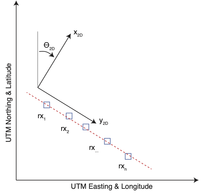
Fig. 36 UTM coordinates and MARE2DEM’s x and y coordinates for an arbitrary receiver array (blue squares) along a survey profile (red dashed line). \(\theta_{2D}\) is the angle between geographic north and the strike direction x of the 2D model. MT impedance tensors should be rotated so that receiver x is aligned with \(x_{2D}\) and then the 2D TE mode is the \(Z_{xy}\) component and the TM mode is the \(Z_{yx}\) component. Likewise, marine CSEM data should be rotated so that a normal linear transmitter tow profile is along the 2D y axis (i.e. across the 2D strike) and thus the inline horizontal electric field will be the \(E_y\) component (after rotating the data to the 2D axes).

Note

In the sections below, we denote angles using units of degrees rather than radians. Make sure your computations use the correct units for the trigonometric functions called upon. MATLAB has trigonometric function names that end with the letter d and these expect input arguments (or output arguments for the inverse functions) have units of degrees (see \(\mathrm{cosd,sind,tand}\)), whereas the \(\cos,\sin,\tan\) functions is radian units.

2D Model Strike Angle

The model strike angle \(\theta_{2D}\) should be determined first. This is the angle from geographic north to the 2D model strike (i.e., MARE2DEM’s x direction). There are a two main ways to determine this angle.

1. If the UTM eastings and northings are stored in arrays E and N and the n receivers are in a straight line, the strike angle is then simply found by the line defined by differencing the locations of two receivers. Using the first and last receivers gives:

   \[\begin{split}\begin{eqnarray} \Delta E &=& E_n- E_1 \\ \Delta N &=& N_n - N_1 \\ \theta_{2D} &=& -\mathrm{atan2d}(\Delta N ,\Delta E) \end{eqnarray}\end{split}\]

   For example, the line in Fig. 36 has \(\theta_{2D}=\) 45º and thus the receiver data can be rotated so x points along 45º and y points along 135º

2. If the receivers aren’t in a perfectly straight line, the least squares method can be used to fit a line to the northing and easting data with:

   \[\begin{eqnarray} N_i = m \, E_i + b, \;\;\; \mathrm{for}\;\;i=1,...n, \end{eqnarray}\]

   and solving for the slope m and intercept b. Then

   \[\begin{eqnarray} \theta_{2D} &=& -\mathrm{atand}(m) + c \end{eqnarray}\]

   where c can be either 0º or 180º to put the strike in the desired direction.

Projecting UTM onto Model x,y

After determining \(\theta_{2D}\), the UTM coordinates must be projected onto model x and y coordinates. First pick a reference UTM location for \((N_0,E_0)\); this will also be where x=0,y=0 in MARE2DEM’s coordinates. We recommend making this either the first receiver, the middle of the array, or some other place along the model profile. The MARE2DEM coordinates are then computed from the UTM coordinates using:

\[\begin{split}\begin{eqnarray} x_{i} &=& \;\;(N_i - N_0) \cos \theta_{2D} + (E_i - E_0) \sin \theta_{2D} \\ y_{i} &=&-(N_i - N_0) \sin\theta_{2D} + (E_i - E_0) \cos \theta_{2D} \end{eqnarray}\end{split}\]

or in matrix notation as

\[\begin{split}\begin{eqnarray} \left[\begin{array}{r} x_i \\ y_i \end{array}\right] &=& \left[\begin{array}{rr} \cos \theta_{2D} & \sin \theta_{2D} \\ -\sin \theta_{2D} & \cos \theta_{2D}\end{array}\right] \left[\begin{array} {r} (N_i - N_0) \\ (E_i - E_0) \end{array}\right]. \end{eqnarray}\end{split}\]

If \((N_0,E_0)\) is chosen to be on the profile, \(x_i\) will be negligibly small or zero for receivers deployed close to or on the profile. \(y_i\) will correspond to along profile distance relative to the origin.

Rotating Vector Data

Vector electric and magnetic field CSEM responses can be rotated from arbitrary recording directions to the MARE2DEM coordinate system, using the vector rotation:

\[\begin{split}\begin{eqnarray} \left[\begin{array}{r} E_x \\ E_y \end{array}\right] &=& \left[\begin{array}{rr} \cos \theta & \sin \theta \\ -\sin \theta & \cos \theta \end{array}\right] \left[\begin{array}{r} E_{x'} \\ E_{y'} \end{array}\right], \end{eqnarray}\end{split}\]

where \(E_{x'}\) and \(E_{y'}\) are the vectors components as recorded in the field along orthogonal axes x’ and y’. The rotation angle \(\theta\) is

(1)\[\theta = \theta_{2D} - (\theta_{x'} + \theta_{D}),\]

where \(\theta_{x'}\) is the geomagnetic orientation angle of recording direction x’ and \(\theta_{D}\) is the geomagnetic declination and \(\theta_{2D}\) is the MARE2DEM strike direction (x axis). Note that \(\theta\) is a relative angle; it is the amount of rotation to apply to move the vector from the recording axes to the MARE2DEM coordinate axes.

The rotation can be written in matrix notation as

\[\mathbf{E}_{2D} = \mathbf{R} \, \mathbf{E}'.\]

Note

Pay attention to how your data rotation software works. In the sections here, \(\theta\) is a relative rotation angle to apply to the data. However, many software programs will request the absolute angle (i.e. the direction to rotate the data to), which here is \(\theta_{2D}\), and then internally these programs apply the relative rotation angle.

Rotating MT Impedance tensors

The \(2 \times 2\) MT impedance tensor can be rotated using the expression

\[\mathbf{Z}_{2D} = \mathbf{R} \, \mathbf{Z}' \, \mathbf{R}^{-1},\]

which in expanded form is

\[\begin{split}\begin{eqnarray} \left[\begin{array}{rr} Z_{xx} & Z_{xy} \\ Z_{yx} & Z_{yy} \end{array}\right] &=& \left[\begin{array}{rr} \cos \theta & \sin \theta \\ -\sin \theta & \cos \theta \end{array}\right] \left[\begin{array}{rr} Z_{x'x'} & Z_{x'y'} \\ Z_{y'x'}' & Z_{y'y'} \end{array}\right] \left[\begin{array}{rr} \cos \theta & -\sin \theta \\ \sin \theta & \cos \theta \end{array}\right] . \end{eqnarray}\end{split}\]

where \(\theta\) is defined in (1).

Why does the impedance get left and right multiplied by the rotation matrix? This is because the impedance relates the electric and magnetic field vectors and each vector has to be rotated, as is shown in the following:

\[\begin{split}\begin{eqnarray} \mathbf{E}_{2D} &=& \mathbf{Z}_{2D} \, \mathbf{H}_{2D} \\ \mathbf{R} \, \mathbf{E}' &=& \mathbf{Z}_{2D} \mathbf{R} \, \mathbf{H}' \\ \mathbf{E}' &=& \mathbf{R}^{-1} \mathbf{Z}_{2D} \mathbf{R} \, \mathbf{H}' \\ &=& \mathbf{Z}' \mathbf{H}' \end{eqnarray}\end{split}\]

so

\[\begin{eqnarray} \mathbf{Z}' &=& \mathbf{R}^{-1} \mathbf{Z}_{2D} \mathbf{R}, \end{eqnarray}\]

and

\[\begin{eqnarray} \mathbf{Z}_{2D} &=& \mathbf{R} \mathbf{Z}' \mathbf{R}^{-1}. \end{eqnarray}\]

Geographic to Polar Stereographic to MARE2DEM

This section describes how to convert data collected in polar regions onto the x and y coordinates axes used in MARE2DEM and was written after we collected the SALSA EM data set in Antarctica.

UTM zones are not defined for the polar regions and instead a polar stereographic grid is used to project the geographic coordinates onto a flat surface. See Fig. 37.

Latitude and longitude should be converted into polar stereographic \(x_{ps}\) and \(y_{ps}\) coordinates using a suitable conversion tool. Note that polar stereographic coordinates use z positive up, so \(y_{ps}\) points upward on the figure and \(x_{ps}\) points to the right (this is the reverse of MARE2DEM’s x and y coordinates). The origin of the polar stereographic grid is at the pole (north or south). Polar stereographic coordinates can be then projected onto MARE2DEM’s (x,y) coordinate system, as shown in the figure below. Rotating the data to MARE2DEM’s (x,y) axes is more difficult for the polar stereographic projection since the direction to geographic north varies across the polar stereographic grid, as can be seen in the figure below. Thus, each station’s data will have a unique rotation angle, depending on its position on the polar stereographic grid. The steps required are described in more detail below.

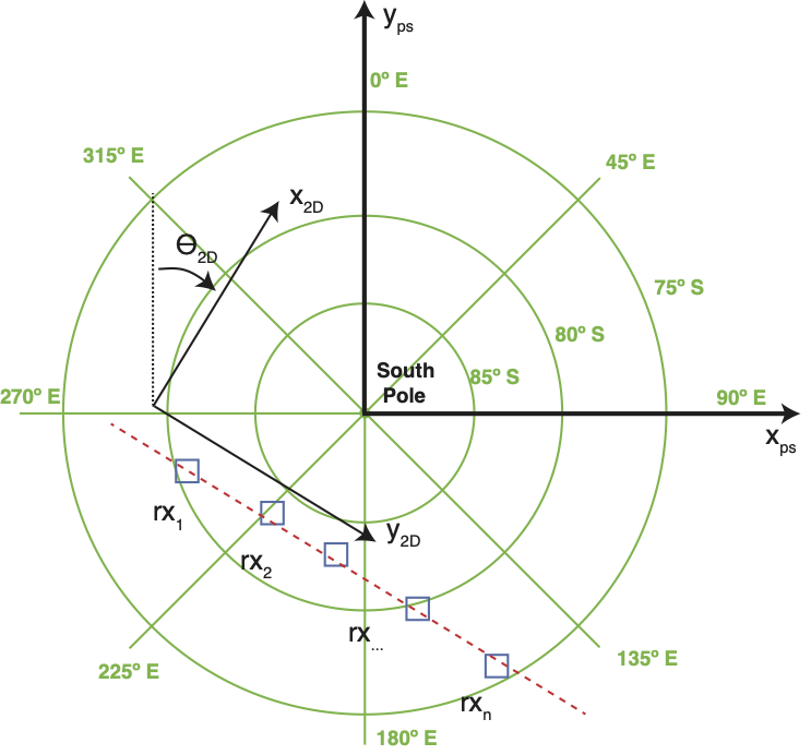
Fig. 37 Geographic (green lines for longitude and latitude), polar stereographic (\(x_{ps}\) and \(y_{ps}\)) and MARE2DEM’s 2D x and y coordinates. Note that polar stereographic coordinates are right handed with z pointing up, so \(x_{ps}\) and \(y_{ps}\) are reversed from MARE2DEM’s coordinates. Green radial lines of longitude point outward towards geographic north (and inward to the south pole). For this hypothetical large scale polar array of receivers (blue squares), the angles from geographic north to \(y_{ps}\) will be substantially different for each receiver and thus each receiver will have a unique rotation angle to rotate its EM data into the MARE2DEM x,y reference frame.

2D Model Strike Angle for Polar Stereographic Coordinates

The 2D model strike (i.e., the model’s x direction) relative to polar stereographic \(y_{ps}\) can be determined in one of two ways.

1. For n receivers in a straight line, the strike angle is found by differencing the locations of the first and last receivers:

   \[\begin{split}\begin{eqnarray} \Delta x_{ps} &=& x_{ps,n}-x_{ps,1} \\ \Delta y_{ps} &=& y_{ps,n}-y_{ps,1} \\ \theta_{2D} &=&-\mathrm{atan2d}(\Delta y_{ps} ,\Delta x_{ps}) \end{eqnarray}\end{split}\]

2. If the receivers aren’t in a perfectly straight line, the least squares method can be used to fit a line to the \(x_{ps}\) and \(y_{ps}\) data with:

   \[\begin{eqnarray} y_{ps,i} = m \, x_{ps,i} + b, \;\;\; \mathrm{for}\;\; i=1,...n, \end{eqnarray}\]

   and solving for the slope m and intercept b. Then

   \[\begin{eqnarray} \theta_{2D} &=& -\mathrm{atand}(m) + c \end{eqnarray}\]

   where c is either 0º or 180º to put the strike in the desired direction.

Projecting Polar Stereographic onto Model x,y

After determining \(\theta_{2D}\), the polar stereographic coordinates (\(x_{ps},y_{ps}\)) are projected onto MARE2DEM’s x and y axes. Pick a reference location (\(x_{ps,0},y_{ps,0}\)) for the origin where x=0,y=0 in MARE2DEM. We recommend making this either the first receiver, the middle of the array, or some other place along the model profile. The MARE2DEM coordinates are then

\[\begin{split}\begin{eqnarray} x_{i} &=& \;\; (y_{ps,i} - y_{ps,0}) \cos \theta_{2D} + (x_{ps,i} - x_{ps,0}) \sin \theta_{2D} \\ y_{i} &=&-(y_{ps,i} - y_{ps,0}) \sin \theta_{2D} + (x_{ps,i} - x_{ps,0}) \cos \theta_{2D} \end{eqnarray}\end{split}\]

or in matrix notation as

\[\begin{split}\begin{eqnarray} \left[\begin{array}{r} x_i \\ y_i \end{array}\right] &=& \left[\begin{array}{rr} \cos \theta_{2D} & \sin \theta_{2D} \\ -\sin \theta_{2D} & \cos \theta_{2D} \end{array}\right] \left[\begin{array}{r} (y_{ps,i} - y_{ps,0})\\ (x_{ps,i} - x_{ps,0}) \end{array}\right]. \end{eqnarray}\end{split}\]

If \(x_{ps,0},y_{ps,0}\) is chosen to be on the profile, \(x_i\) will be negligibly small or zero for receivers deployed close to or on the profile. \(y_i\) will correspond to along profile distance relative to the origin.

Receiver Rotations for Polar Stereographic Coordinates

For polar stereographic coordinates, each receiver can have a different rotation angle depending on its position on the stereographic grid. This can be seen in Fig. 38, where it is clear that for each receiver there is a different angle between \(y_{ps}\) and geographic north.

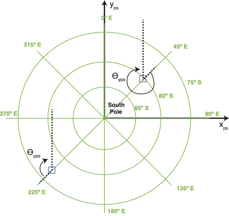
Fig. 38 The angle \(\theta_{yps}\) is the angle from geographic north to the \(y_{ps}\) axis. Note that each receiver may have a different \(\theta_{yps}\).

The angle \(\theta_{yps}\) is the angle from geographic north to the \(y_{ps}\) axis at each receiver, as shown in the figure below. For a given receiver with position \((x_{ps},y_{ps})\), the angle \(\theta_{yps}\) can be computed using

\[\begin{eqnarray} \theta_{yps} = -\mathrm{atan2d}(x_{ps},y_{ps}). \end{eqnarray}\]

Now we can define the specific rotation for each receiver’s data. This is the relative angle that receiver’s data should be rotated by so that it is aligned with MARE2DEM’s (x,y) axes. Since \(\theta_{yps}\) is the angle from geographic north to \(y_{ps}\) and \(\theta_{2D}\) is the angle from \(y_{ps}\) to the 2D model’s x and y axes, the receiver’s vector data should be rotated by the angle:

\[\begin{eqnarray} \theta = \theta_{yps} + \theta_{2D} - (\theta_{x'} + \theta_{D}), \end{eqnarray}\]

where \(\theta_{x'}\) is the geomagnetic orientation angle of recording direction x’ and \(\theta_{D}\) is the geomagnetic declination. For typical land MT recordings, the sensors are oriented using a compass so that x’ points to geomagnetic north and hence \(\theta_{x'} = 0\). And again, note that \(\theta\) is the relative angle to rotate the data by. If instead your software requests, the absolute angle to rotate the data to, then use the absolute angle: \(\theta_{yps} + \theta_{2D}\) (assuming the declination correction has been applied).