This section gives a brief overview of the typical workflow for
MARE2DEM. The suite of MARE2DEM codes consists of three parts:
A MATLAB user interface and other routines for building forward and
inverse model and preparing data files
The core MARE2DEM code (written in MPI-Fortran and C) for the finite
element modeling and inversion of EM responses
MATLAB routines for interactive plotting of inversion models and viewing
EM responses and data fits
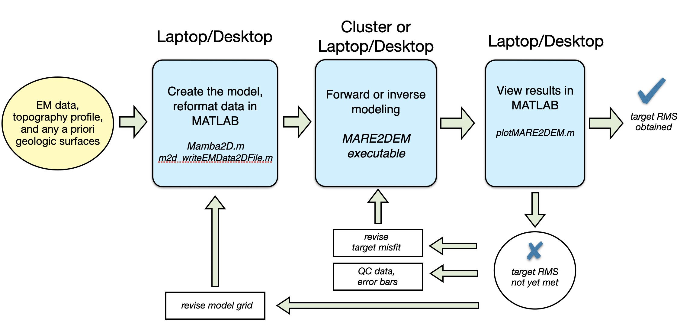
The typical workflow is outline in the image below:
Input data consists of the transmitters and receivers and response frequencies and
any topography and other geologic surfaces that will be incorporated into the model.
In MATLAB, the data parameters (and any EM responses to be inverted) can be written to a
MARE2DEM format data file using m2d_writeEMData2DFile.m.
A resistivity model (and possibly an inversion mesh) is built using the interactive
Mamba2D.m graphical user interface.
The MARE2DEM executable code is run for forward or inverse modeling.
Results are viewed in MATLAB using plotMARE2DEM.m.
For inversion, the resulting model and data fits are inspected and if
deemed insufficient, the model parameterization is revised and outlier
or noisy data are trimmed and the workflow is repeated.
There are four input files required to run MARE2DEM for forward
modeling; a fifth file is needed for inversion. They are all created by
Mamba2D.m except for the data file. For a model named demo, the
following files are needed:
demo.0.resistivity specifies the resistivity of each model
parameter region and whether or not the parameter is fixed or an inversion free
parameter, the resistivity anisotropy setting, inversion parameter resistivity bounds
and prejudices (if any), and lists the names of the other required files.
The file extension 0 specifies the inversion iteration number; 0 means this is is a starting
model. When running inversions, a new resistivity file is output for
each iteration of the inversion and this number will indicate the
inversion iteration.
demo.poly specifies the geometry of the model parameter grid (nodes and segments connecting them)
demo.penalty contains the inversion’s roughness penalty matrix (only needed for inversion).
demo.emdata specifies the sources, receivers and frequencies to be
modeled as well the type of data and any real data to be inverted.
mare2dem.settings specifies various runtime settings for MARE2DEM, including the
accuracy tolerance for EM responses generated by the automatic
adaptive mesh refinement, and how the data should be decomposed into
subsets for parallel computations.
See the section File Formats section for further details.
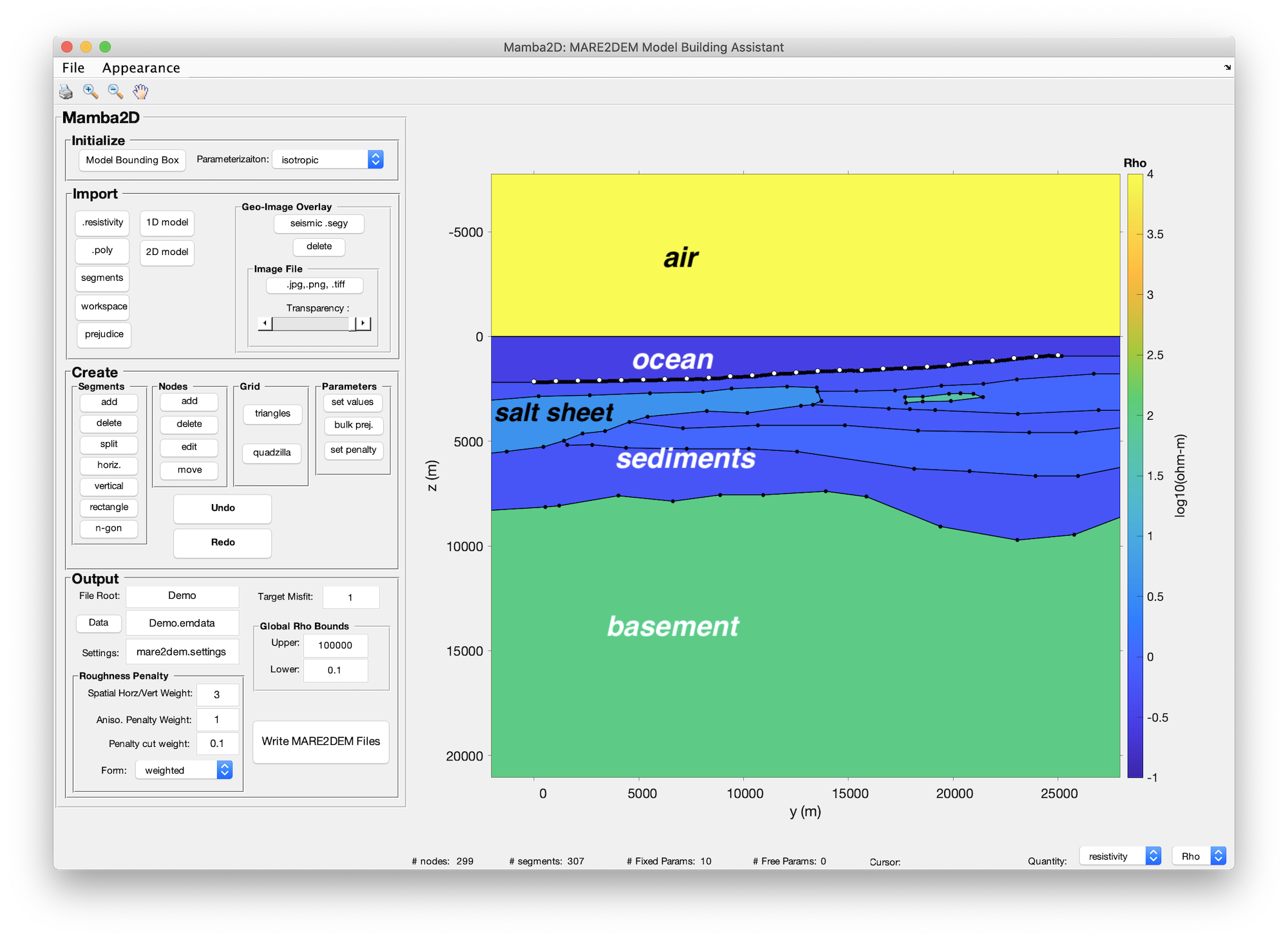
Fig. 1 Example forward modeling mesh for the demo example created
with the interactive Mamba2D.m graphical user interface. The
model consists of nodes that are connected by line segments. These
nodes and segments define the model geometry and are stored in the
.poly file. Each segment bound polygonal region is assigned a unique
resistivity value. You can draw model regions interactively by
pointing and clicking, or by importing surface profiles
(position,depth) and connecting them. Hitting the WriteMARE2DEMFiles button then creates the .resistivity, .poly and .settings
files. Then entire model extends 100 km in each direction and here
only the central region of interest is shown.
Note
No meshing or gridding is needed for forward modeling. Just draw the
desired model structure and assign resistivity values to each
segment bound region, save the files and let MARE2DEM do the rest.
When you run MARE2DEM, it will load in the model that you created
with Mamba2D.m and then MARE2DEM automatically generates
adaptive finite element meshes that conform to the model geometry
and that are iteratively refined to give accurate EM responses for
the particular transmitters and receivers being modeled. All finite
element meshing and refinement in MARE2DEM is done internally behind
the scenes while it runs and these dynamically generated meshes are
not saved to files.
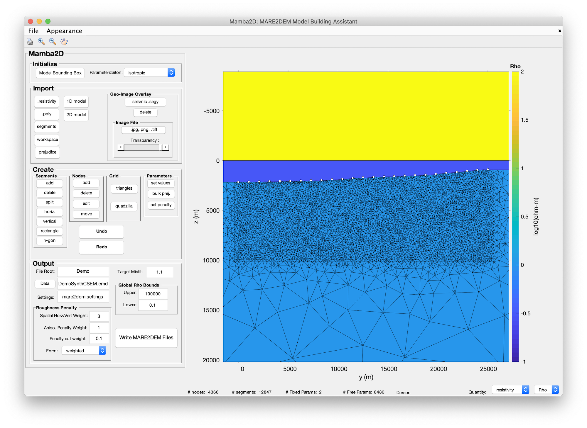
Fig. 2 Example inversion modeling grid for the demo example. For
inversion, the model starts with three layers (air,sea, seafloor)
and the seafloor region is assigned to be a free parameter. A region
of interest box is created beneath the seafloor and is filed with
a triangular mesh of model parameters with a target size. The outer
padding region is also meshed with arbitrarily larger triangles. The
inversion will then solve for the resistivity of these triangular
parameters. Note that the any polygonal region can be a free
parameter for inversion; here we used triangles since Mamba2D has a
versatile unstructured triangular meshing engine that can mesh
complicated regions, but we could have also used quadrilateral or
other polygon shapes for the parameter grid. Only the central region
of interest is shown in this image.
After the input files have been created, MARE2DEM can be run locally on
your laptop or desktop if the modeling problem is small (a MT data
set or a small CSEM problem), or the files can be transferred to a HPC
cluster where MARE2DEM is run remotely (e.g., for large CSEM data
sets).
Fig. 3 Example startup of MARE2DEM for the demo example on a
MacBook Pro with 8 processing cores. Here I opened a terminal, cd’d
to the demo folder and listed in contents using ls. You can see
the five required input files are there. Then I launch MARE2DEM using
mpirun command with the argument -n8, which tells MPI to
use 8 processors. The MARE2DEM executable is followed by the
name of the resistivity file to start the inversion with, here
Demo.0.resistivity.
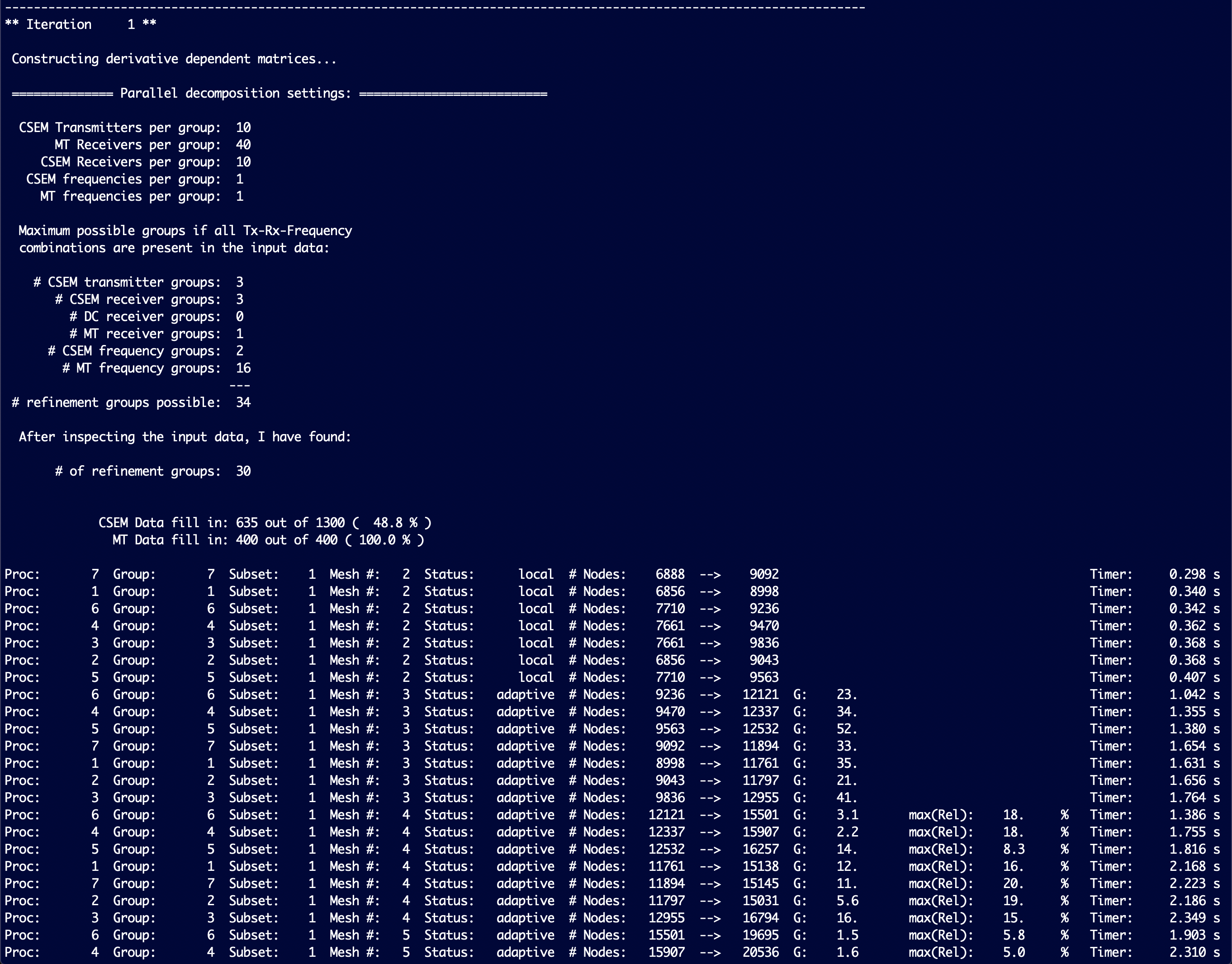
Fig. 4 Example showing some runtime output of MARE2DEM for the demo
example. The text on the lower half shows the adaptive mesh
refinement details for various data subsets as the parallel
calculations proceed. For inversion runs of MARE2DEM, the
convergence history of each iteration is saved to a separate
.logfile file so you can easily monitor its progress.
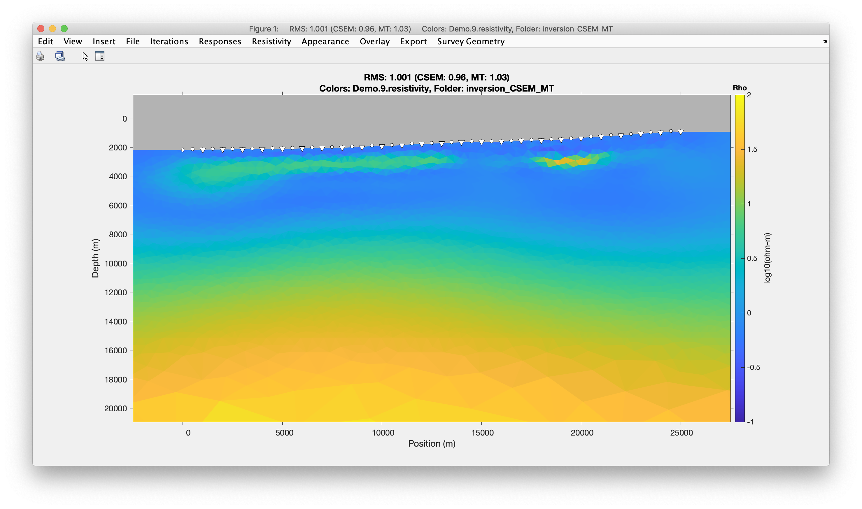
Fig. 5 Example showing the inversion result for the demo example of
that has synthetic MT and CSEM data generated from the forward model
shown above. The inversion model was plotted in MATLAB using
MARE2DEM’s code plotMARE2DEM.m, which allows for interactive
exploration of the model results.
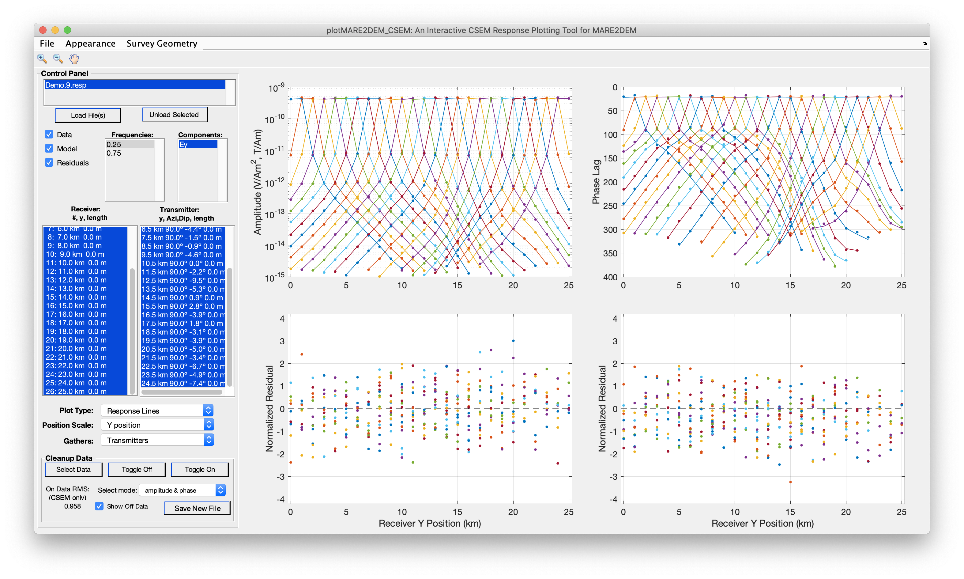
Fig. 6 Example showing the inversion fit to the CSEM data for the demo example plotted in
MATLAB using MARE2DEM’s code plotMARE2DEM_CSEM.m.
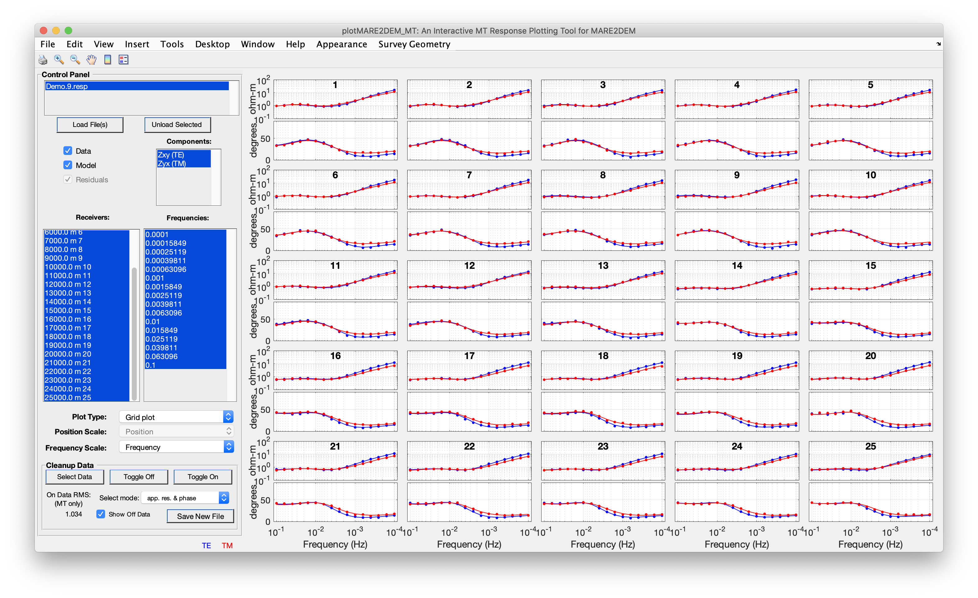
Fig. 7 Example showing the inversion fit to the MT data for the demo example plotted in
MATLAB using MARE2DEM’s code plotMARE2DEM_MT.m.
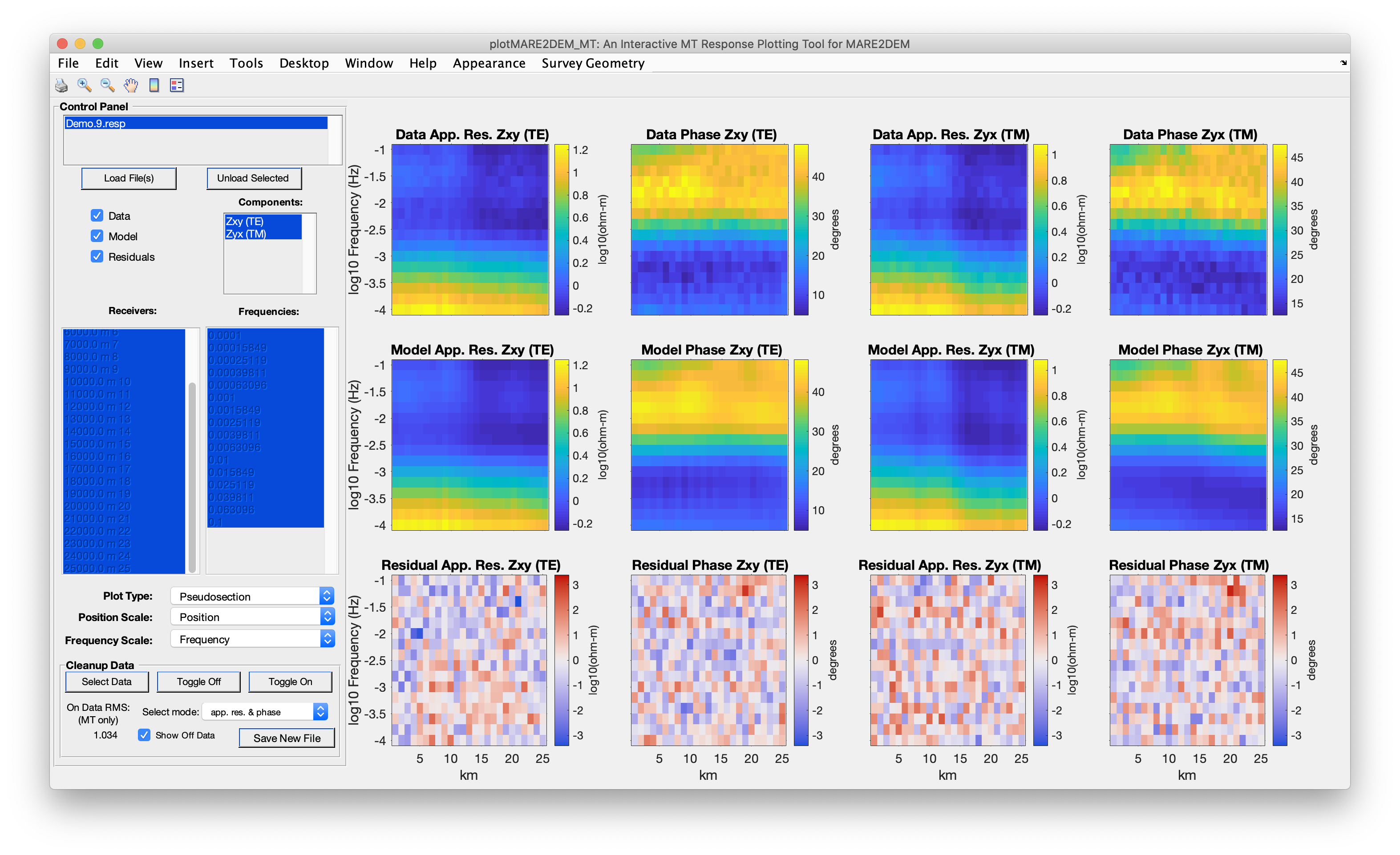
Fig. 8 Example pseudosection plot showing the inversion fit to the MT
data for the demo example, made with plotMARE2DEM_MT.m.
You can see a nice fit to the data, and in this ideal synthetic
example, the normalized residuals have a nice random distribution.
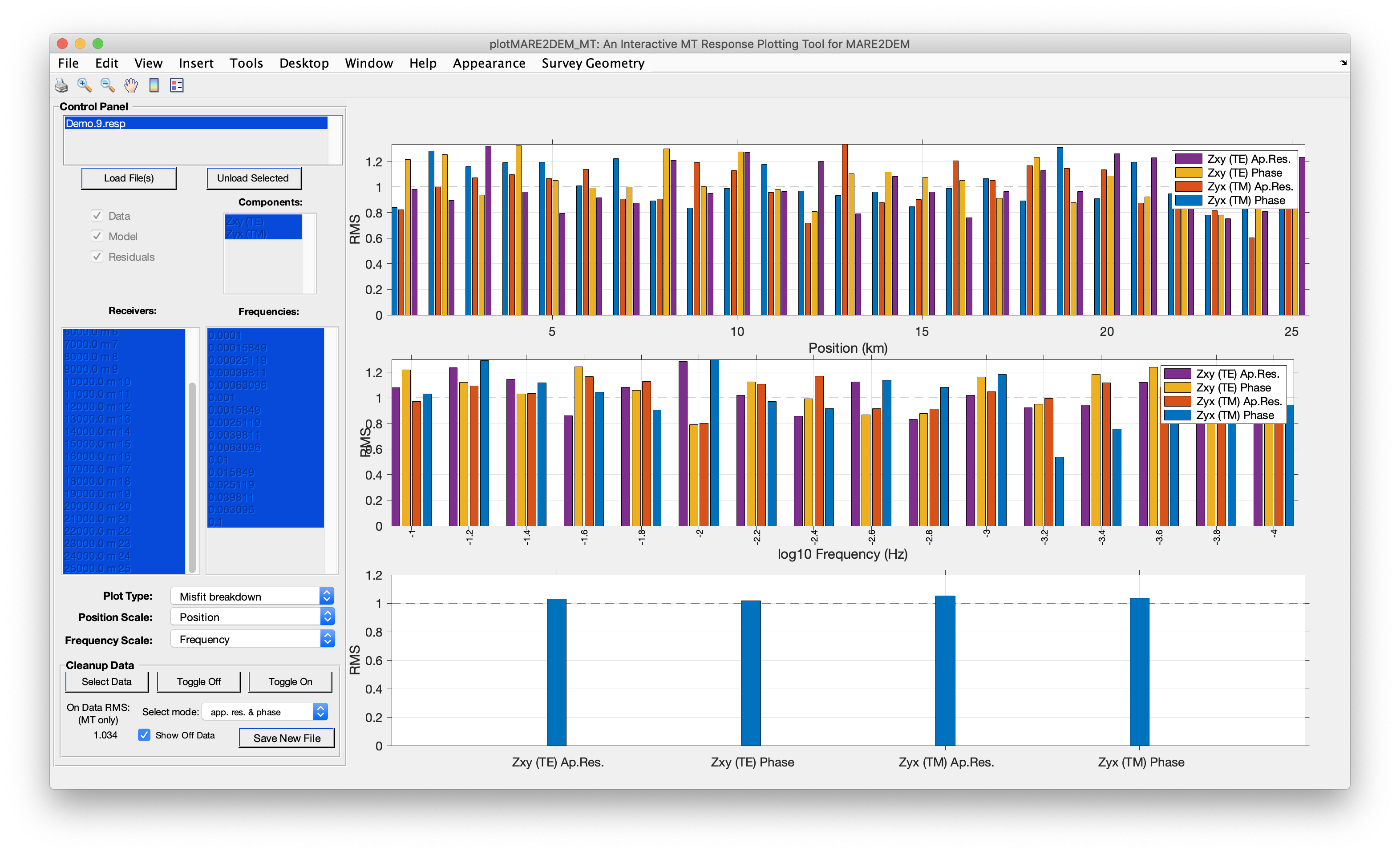
Fig. 9 Example MT misfit-breakdown plot for the inversion fit to the MT
data for the demo example, made using plotMARE2DEM_MT.m.
In this ideal synthetic example, you can see that no matter how we
slice-and-dice the MT data, the various subsets have RMS misfits
close to the target 1.0 value, suggesting the model is a good
overall fit to the MT stations.